Difference between revisions of "Modeling Human Performance"
User:Fellrnr (User talk:Fellrnr | contribs) m (Fellrnr moved page Training Stress Balance to Modeling Human Performance) |
User:Fellrnr (User talk:Fellrnr | contribs) |
||
| (3 intermediate revisions by the same user not shown) | |||
| Line 1: | Line 1: | ||
| − | + | There are a number of approaches to modeling how training changes performance and these models have some obvious value in optimizing a training routine, especially for tapering. | |
| − | + | =The Models= | |
| − | =TSB | + | The models assume that given training stress, also known as "training impulse" or [[TRIMP]] ('''TR'''aining '''IMP'''ulse), has both a positive and a negative effect. The positive effect is called "fitness", and the negative effect is called "fatigue", and they are combined to provide a value of "performance". This article looks at three models: |
| + | * Banister. The initial work on modeling human performance was made by Eric Banister in 1975<ref name="CalvertBanister1976"/> and verified by dozens of studies including one on runners<ref name="Morton-1990"/>. | ||
| + | * Busso. The work of Banister was refined by Thierry Busso to modify the Banister model to at least partly account for how [[Training Monotony]] impacts recovery<ref name="Busso-2003"/>. | ||
| + | * TSB. The Training Stress Balance model is a simplification of the Banister model by Andrew Coggan which looks at just the relative changes in performance<ref name="TSB"/>. | ||
| + | The TSB model will be examined first, as it's the simplest to understand. | ||
| + | =The TSB Model= | ||
| + | Training Stress Balance (TSB) uses the terms Chronic Training Load (CTL) for "fitness", Acute Training Load (ATL) for "fatigue" and Training Stress Balance (TSB) for "performance". As with all the models, both CTL and ATL are based on TRIMP, with the effect of a given workout reducing over time, but the effect lasts longer on CTL than on ATL. In addition the TSB method assumes the effect is greater on CTL than on ATL. | ||
| + | ==TSB for a Single Workout== | ||
[[File:TSB Single Workout.jpg|none|thumb|500px]] | [[File:TSB Single Workout.jpg|none|thumb|500px]] | ||
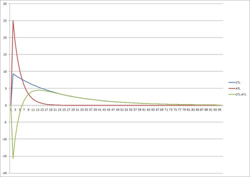
The image above shows the effect of a single workout on the Training Stress Balance. You can see the workout creates a peak in both ATL and CTL. The peak is greater ATL, but reduces more quickly than in CTL. The Training Stress Balance is CTL-ATL, and you can see it initially go negative indicating a reduced ability to perform, then rises to be positive as CTL becomes greater than ATL. This green TSB line is the same as that seen in [[Supercompensation]]. | The image above shows the effect of a single workout on the Training Stress Balance. You can see the workout creates a peak in both ATL and CTL. The peak is greater ATL, but reduces more quickly than in CTL. The Training Stress Balance is CTL-ATL, and you can see it initially go negative indicating a reduced ability to perform, then rises to be positive as CTL becomes greater than ATL. This green TSB line is the same as that seen in [[Supercompensation]]. | ||
| − | + | ==TSB for Multiple Workouts== | |
| − | =TSB for Multiple Workouts= | + | [[File:TSB-KaKfSame.jpg|none|thumb|500px]] |
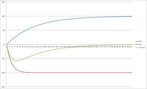
| − | [[File:TSB | + | The effect of a continuous series of identical workouts on TSB is shown in the image above. The ATL rises sharply and reaches a steady-state, with CTL rising more slowly to a greater level. The TSB (CTL-ATL) goes negative, slowly returning to zero. |
| − | The effect of a continuous series of identical workouts on TSB is shown in the image above. The ATL rises sharply and reaches a steady-state, with CTL rising more slowly to a greater level. The TSB (CTL-ATL) | + | ==TSB Constants== |
| − | + | Because the TSB model is simpler than the other two, it only requires the number of days that ATL and CTL decay over. The typical starting point is 7 days for ATL and 42 days for CTL. | |
| − | = | + | ==Calculation Details== |
| − | |||
| − | |||
| − | = | ||
| − | |||
| − | |||
| − | |||
| − | |||
| − | |||
| − | |||
| − | |||
| − | |||
| − | |||
| − | |||
| − | |||
| − | |||
| − | |||
| − | |||
| − | |||
| − | |||
| − | |||
| − | |||
| − | |||
| − | =Calculation Details= | ||
Understanding these details is not required for using the TSB, but you may find them interesting. | Understanding these details is not required for using the TSB, but you may find them interesting. | ||
| − | + | ===The TSB Formulas=== | |
| − | ==The | ||
The basic formula for calculating ATL/CTL uses an [http://en.wikipedia.org/wiki/Moving_average\#Exponential_moving_average Exponential moving average] that is calculated like this: | The basic formula for calculating ATL/CTL uses an [http://en.wikipedia.org/wiki/Moving_average\#Exponential_moving_average Exponential moving average] that is calculated like this: | ||
| − | ATL<sub>today</sub> = [[TRIMP]] * λ | + | ATL<sub>today</sub> = [[TRIMP]] * λ<sub>a</sub> + ((1 – λ<sub>a</sub>) * ATL<sub>yesterday</sub> |
| − | CTL<sub>today</sub> = [[TRIMP]] * λ | + | CTL<sub>today</sub> = [[TRIMP]] * λ<sub>f</sub> + ((1 – λ<sub>f</sub>) * CTL<sub>yesterday</sub> |
| − | As you can see this is an iterative approach, calculating the value for the oldest workout, then iterating through each subsequent workout. | + | As you can see this is an iterative approach, calculating the value for the oldest workout, then iterating through each subsequent workout. The calculation for λ<sub>a</sub> and λ<sub>f</sub> is: |
| − | |||
| − | |||
| − | The calculation for λ<sub>a</sub> and λ<sub>f</sub> is: | ||
λ<sub>a</sub> = 2/(N<sub>a</sub>+1) | λ<sub>a</sub> = 2/(N<sub>a</sub>+1) | ||
λ<sub>f</sub> = 2/(N<sub>f</sub>+1) | λ<sub>f</sub> = 2/(N<sub>f</sub>+1) | ||
Where N<sub>a</sub> and N<sub>f</sub> are the time decay constants, normally 7 and 42 days respectively. The [http://en.wikipedia.org/wiki/Half-life half-life] for a given value of N is N/2.8854, so 7 days gives a half-life of 2.4 days and 42 days is 14.5 days. | Where N<sub>a</sub> and N<sub>f</sub> are the time decay constants, normally 7 and 42 days respectively. The [http://en.wikipedia.org/wiki/Half-life half-life] for a given value of N is N/2.8854, so 7 days gives a half-life of 2.4 days and 42 days is 14.5 days. | ||
| − | + | ==Limitations of the TSB model== | |
| − | == | + | The main limitation of the TSB model can be seen in the graph above, which shows that training reduces performance and never improves it. The TSB model only indicates an improved performance when training is reduced, as shown below. |
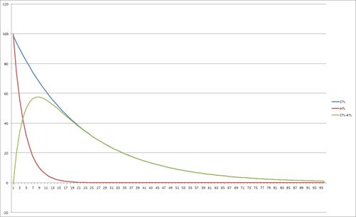
| − | The | + | [[File:TSB-ReducedTraining.jpg|none|thumb|500px|The TSB model when training is reduced from a stable level of 100 TRIMP per day to zero, showing the rapid drop in fatigue (ATL) and the slower drop in fitness (CTL), resulting in an improved performance (TSB).]] |
| − | + | =The Banister Model= | |
| − | == | + | The Banister model is a little more complex mathematically than TSB, using an exponential decay to model the effects of training stress. Unlike the TSB model, the Banister model will show that a steady state of training will improve performance. Of the available models, Banister's is the most experimentally validated. |
| − | The | + | ==The Banister Formula== |
| − | + | The formula below looks rather complex, but is actually fairly simple to implement. | |
| − | + | [[File:BanisterFormula.jpg|none|thumb|500px]] | |
| − | + | Here it is as some simple pseudo-code for those that want to implement it. | |
| − | + | fitness = 0; | |
| − | + | TRIMP[] = getDailyTRIMP(); //array of TRIMP for each day | |
| − | + | for(i=0, i < count(TRIMP); i++) | |
| − | + | { | |
| − | + | fitness = fitness * exp(-1/r1) + TRIMP[i]; | |
| − | + | fatigue = fatigue * exp(-1/r2) + TRIMP[i]; | |
| − | === | + | performance = fitness * k1 - fatigue * k2; |
| − | + | } | |
| − | + | This model uses four constants. | |
| − | + | * k1 is a positive weighting constant for fitness. | |
| − | + | * k2 is a positive weighting constant for fatigue, with | |
| − | + | * A larger k1 than k2 indicates an individual takes longer to recover, whereas a larger k2 than k1 indicates a faster recovery. | |
| − | + | * r1 is the time decay for fitness in days (how long does it take for fitness to return to baseline). | |
| − | + | * r2 is the time decay for fatigue in days (how long does it take for fatigue to return to baseline). | |
| + | * Because fitness lasts longer than fatigue, r1 is larger (longer) than r2. | ||
| + | * The original paper used values of k1=1.0, k2=1.8-2.0, r1=49-50, r2=11. | ||
| + | =The Busso Model= | ||
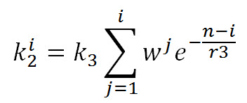
| + | Thierry Busso created a refinement of the Banister model to try to take account of how an increase in [[Training Monotony]] also increased fatigue. This modification of Banister changes k2 from being a constant to being an exponential decay of the training stress. | ||
| + | [[File:BussoMainFormula.jpg|none|thumb|500px]] | ||
| + | The value of k2 uses a similar exponential decay: | ||
| + | [[File:BussoK2Formula.jpg|none|thumb|500px]] | ||
| + | =Flaws in the models= | ||
| + | There are a number of practical flaws in these models. | ||
| + | * The main flaw with these models is that the values for the constants used are specific to each individual, and possibly to the particular training regime. The verification of the Banister and Busso models reverse engineered the constants so that the model accurately predicted the performance changes. | ||
| + | * The values of the constants and the resulting predictions also depend on the performance metric being used. | ||
| + | * Another flaw is that the models assume a single value for that represents the adaptation to performance. In practice, different types of adaptation occur at different rates. | ||
| + | * The TSB and Banister models ignore [[Overtraining]] & [[Training Monotony]] and predict that any possible workload produces improved fitness. | ||
| + | * The TSB model assumes that training does not produce an improved performance. Instead the TSB model only detects a change in training level, with reduced training improving performance and increased training reduces performance. | ||
| + | =Comparison of the Models= | ||
| + | * The TSB model is simpler than the other two models as it only has the two decay parameters. | ||
| + | * The Banister model has more experimental verification than the other models. | ||
| + | * The Busso model is the most complex, but is the only one that allows for [[Training Monotony]]. | ||
| + | =Implementing the Models= | ||
| + | These three models are implemented in the free [[SportTracks Dailymile Plugin]]. | ||
| + | =References= | ||
| + | <references> | ||
| + | <ref name="Morton-1990"> RH. Morton, JR. Fitz-Clarke, EW. Banister, Modeling human performance in running., J Appl Physiol, volume 69, issue 3, pages 1171-7, Sep 1990, PMID [http://www.ncbi.nlm.nih.gov/pubmed/2246166 2246166]</ref> | ||
| + | <ref name="CalvertBanister1976">Thomas W. Calvert, Eric W. Banister, Margaret V. Savage, Tim Bach, A Systems Model of the Effects of Training on Physical Performance, IEEE Transactions on Systems, Man, and Cybernetics, volume SMC-6, issue 2, 1976, pages 94–102, ISSN [http://www.worldcat.org/issn/0018-9472 0018-9472], doi [http://dx.doi.org/10.1109/TSMC.1976.5409179 10.1109/TSMC.1976.5409179]</ref> | ||
| + | <ref name="Busso-2003"> T. Busso, Variable dose-response relationship between exercise training and performance., Med Sci Sports Exerc, volume 35, issue 7, pages 1188-95, Jul 2003, doi [http://dx.doi.org/10.1249/01.MSS.0000074465.13621.37 10.1249/01.MSS.0000074465.13621.37], PMID [http://www.ncbi.nlm.nih.gov/pubmed/12840641 12840641]</ref> | ||
| + | <ref name="TSB"> TrainingPeaks, http://www.peaksware.com/articles/cycling/the-science-of-the-performance-manager.aspx, Accessed on 11 May 2013</ref> | ||
| + | </references> | ||
Latest revision as of 09:30, 16 May 2016
There are a number of approaches to modeling how training changes performance and these models have some obvious value in optimizing a training routine, especially for tapering.
Contents
[hide]1 The Models
The models assume that given training stress, also known as "training impulse" or TRIMP (TRaining IMPulse), has both a positive and a negative effect. The positive effect is called "fitness", and the negative effect is called "fatigue", and they are combined to provide a value of "performance". This article looks at three models:
- Banister. The initial work on modeling human performance was made by Eric Banister in 1975[1] and verified by dozens of studies including one on runners[2].
- Busso. The work of Banister was refined by Thierry Busso to modify the Banister model to at least partly account for how Training Monotony impacts recovery[3].
- TSB. The Training Stress Balance model is a simplification of the Banister model by Andrew Coggan which looks at just the relative changes in performance[4].
The TSB model will be examined first, as it's the simplest to understand.
2 The TSB Model
Training Stress Balance (TSB) uses the terms Chronic Training Load (CTL) for "fitness", Acute Training Load (ATL) for "fatigue" and Training Stress Balance (TSB) for "performance". As with all the models, both CTL and ATL are based on TRIMP, with the effect of a given workout reducing over time, but the effect lasts longer on CTL than on ATL. In addition the TSB method assumes the effect is greater on CTL than on ATL.
2.1 TSB for a Single Workout
The image above shows the effect of a single workout on the Training Stress Balance. You can see the workout creates a peak in both ATL and CTL. The peak is greater ATL, but reduces more quickly than in CTL. The Training Stress Balance is CTL-ATL, and you can see it initially go negative indicating a reduced ability to perform, then rises to be positive as CTL becomes greater than ATL. This green TSB line is the same as that seen in Supercompensation.
2.2 TSB for Multiple Workouts
The effect of a continuous series of identical workouts on TSB is shown in the image above. The ATL rises sharply and reaches a steady-state, with CTL rising more slowly to a greater level. The TSB (CTL-ATL) goes negative, slowly returning to zero.
2.3 TSB Constants
Because the TSB model is simpler than the other two, it only requires the number of days that ATL and CTL decay over. The typical starting point is 7 days for ATL and 42 days for CTL.
2.4 Calculation Details
Understanding these details is not required for using the TSB, but you may find them interesting.
2.4.1 The TSB Formulas
The basic formula for calculating ATL/CTL uses an Exponential moving average that is calculated like this:
ATLtoday = TRIMP * λa + ((1 – λa) * ATLyesterday
CTLtoday = TRIMP * λf + ((1 – λf) * CTLyesterday
As you can see this is an iterative approach, calculating the value for the oldest workout, then iterating through each subsequent workout. The calculation for λa and λf is:
λa = 2/(Na+1)
λf = 2/(Nf+1)
Where Na and Nf are the time decay constants, normally 7 and 42 days respectively. The half-life for a given value of N is N/2.8854, so 7 days gives a half-life of 2.4 days and 42 days is 14.5 days.
2.5 Limitations of the TSB model
The main limitation of the TSB model can be seen in the graph above, which shows that training reduces performance and never improves it. The TSB model only indicates an improved performance when training is reduced, as shown below.
3 The Banister Model
The Banister model is a little more complex mathematically than TSB, using an exponential decay to model the effects of training stress. Unlike the TSB model, the Banister model will show that a steady state of training will improve performance. Of the available models, Banister's is the most experimentally validated.
3.1 The Banister Formula
The formula below looks rather complex, but is actually fairly simple to implement.
Here it is as some simple pseudo-code for those that want to implement it.
fitness = 0;
TRIMP[] = getDailyTRIMP(); //array of TRIMP for each day
for(i=0, i < count(TRIMP); i++)
{
    fitness = fitness * exp(-1/r1) + TRIMP[i];
    fatigue = fatigue * exp(-1/r2) + TRIMP[i];
    performance = fitness * k1 - fatigue * k2;
}
This model uses four constants.
- k1 is a positive weighting constant for fitness.
- k2 is a positive weighting constant for fatigue, with
- A larger k1 than k2 indicates an individual takes longer to recover, whereas a larger k2 than k1 indicates a faster recovery.
- r1 is the time decay for fitness in days (how long does it take for fitness to return to baseline).
- r2 is the time decay for fatigue in days (how long does it take for fatigue to return to baseline).
- Because fitness lasts longer than fatigue, r1 is larger (longer) than r2.
- The original paper used values of k1=1.0, k2=1.8-2.0, r1=49-50, r2=11.
4 The Busso Model
Thierry Busso created a refinement of the Banister model to try to take account of how an increase in Training Monotony also increased fatigue. This modification of Banister changes k2 from being a constant to being an exponential decay of the training stress.
The value of k2 uses a similar exponential decay:
5 Flaws in the models
There are a number of practical flaws in these models.
- The main flaw with these models is that the values for the constants used are specific to each individual, and possibly to the particular training regime. The verification of the Banister and Busso models reverse engineered the constants so that the model accurately predicted the performance changes.
- The values of the constants and the resulting predictions also depend on the performance metric being used.
- Another flaw is that the models assume a single value for that represents the adaptation to performance. In practice, different types of adaptation occur at different rates.
- The TSB and Banister models ignore Overtraining & Training Monotony and predict that any possible workload produces improved fitness.
- The TSB model assumes that training does not produce an improved performance. Instead the TSB model only detects a change in training level, with reduced training improving performance and increased training reduces performance.
6 Comparison of the Models
- The TSB model is simpler than the other two models as it only has the two decay parameters.
- The Banister model has more experimental verification than the other models.
- The Busso model is the most complex, but is the only one that allows for Training Monotony.
7 Implementing the Models
These three models are implemented in the free SportTracks Dailymile Plugin.
8 References
- Jump up ↑ Thomas W. Calvert, Eric W. Banister, Margaret V. Savage, Tim Bach, A Systems Model of the Effects of Training on Physical Performance, IEEE Transactions on Systems, Man, and Cybernetics, volume SMC-6, issue 2, 1976, pages 94–102, ISSN 0018-9472, doi 10.1109/TSMC.1976.5409179
- Jump up ↑ RH. Morton, JR. Fitz-Clarke, EW. Banister, Modeling human performance in running., J Appl Physiol, volume 69, issue 3, pages 1171-7, Sep 1990, PMID 2246166
- Jump up ↑ T. Busso, Variable dose-response relationship between exercise training and performance., Med Sci Sports Exerc, volume 35, issue 7, pages 1188-95, Jul 2003, doi 10.1249/01.MSS.0000074465.13621.37, PMID 12840641
- Jump up ↑ TrainingPeaks, http://www.peaksware.com/articles/cycling/the-science-of-the-performance-manager.aspx, Accessed on 11 May 2013


