Modeling Human Performance

Training Stress Balance (TSB) is a method for evaluating the effect of training over time. This approach assumes that given training stress, also known as "training impulse" or TRIMP (TRaining IMPulse), has both a positive and a negative effect. The positive effect could be considered "fitness", and the negative effect could be considered "fatigue." The positive effect is called Chronic Training Load (CTL) and the negative effect is called Acute Training Load (ATL). Both CTL and ATL are based on TRIMP, with the effect of a given workout reducing over time, but the effect lasts longer on CTL than on ATL. In addition the TSB method assumes the effect is greater on CTL than on ATL.

1 TSB For a Single Workout

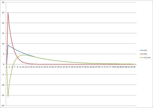
The image above shows the effect of a single workout on the Training Stress Balance. You can see the workout creates a peak in both ATL and CTL. The peak is greater ATL, but reduces more quickly than in CTL. The Training Stress Balance is CTL-ATL, and you can see it initially go negative indicating a reduced ability to perform, then rises to be positive as CTL becomes greater than ATL. This green TSB line is the same as that seen in Supercompensation.

2 TSB for Multiple Workouts

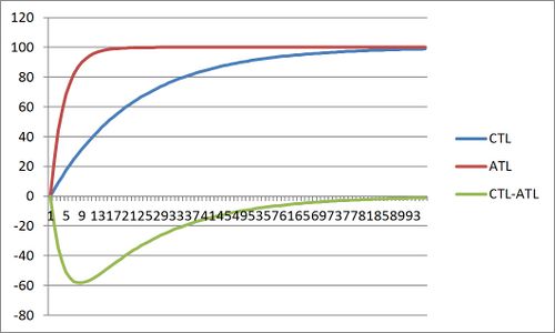
The effect of a continuous series of identical workouts on TSB is shown in the image above. The ATL rises sharply and reaches a steady-state, with CTL rising more slowly to a greater level. The TSB (CTL-ATL) initially goes negative, but rises towards a positive steady-state.

3 The value of the TSB model

The TSB model can provide an estimation of how changes in training load affect fatigue and performance. A positive TSB indicates improved performance.

4 Flaws in the TSB model

There are a number of practical flaws in the TSB model.

• The first flaw in the TSB model is that it ignores Overtraining and predicts that any possible workload produces improved fitness. Related to this problem is that the model ignores Training Monotony. Research has shown that training with a high level of monotony reduces the benefits and increases the fatigue from a given level of training.
• The second flaw is that the values for the constants used in the model are specific to each individual, and possibly to the particular training regime. The verification of the model reverse engineered the constants so that the model accurately predicted the performance changes. These constants are represented below as
  • N_a - the decay constant for acute (fatigue) effect of training.
  • N_f - the decay constant for fitness effect of training.
  • K_a - the scaling constant for acute (fatigue) effect of training
  • K_f - the scaling constant for fitness effect of training.
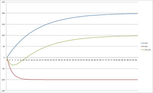
  • The ratio of K_a to K_f defines the benefit of training. If they are both the same value, then you get no benefit from training, but if K_a is larger than K_f then training improves your performance over time.
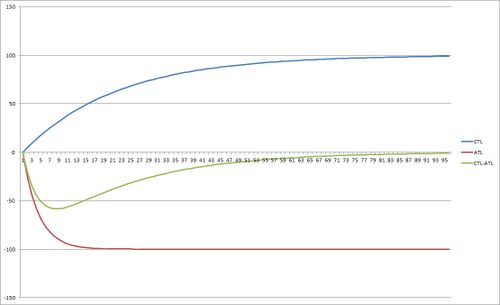
  • If you consider the case of someone starting to exercise exactly the same amount every day, you’d find a change in CTL and ATL that would reach a steady level over time. Without a difference in K_a/K_f, the values of would cancel each other out, so CTL-ATL would be zero, showing no improvement from that exercise. See the graphs below.
• A third flaw is that TSB assumes a single value for that represents the adaptation to performance. In practice, different types of adaptation occur at different rates.

A graph showing someone start an exercise program with the same workout every day. You can see that the TSB (green line) returns to zero, indicating no improvement in performance.

This is the same exercise, but with Kf twice the value of Ka. Now the exercise program predicts an improvement in performance.

5 An Advanced TSB

One approach to addressing these flaws is to use the calculated Training Monotony to change the TSB calculation. Higher levels of monotony should reduce the CTL value, increase the ATL value, and increase the time constant used to reduce the effect of a workout on ATL. I've built this into my SportTracks Dailymile Plugin.

6 Calculation Details

Understanding these details is not required for using the TSB, but you may find them interesting.

6.1 The basic formula

The basic formula for calculating ATL/CTL uses an Exponential moving average that is calculated like this:

ATLtoday = TRIMP * λa * ka + ((1 – λa) * ATLyesterday
CTLtoday = TRIMP * λf * kf + ((1 – λf) * CTLyesterday

As you can see this is an iterative approach, calculating the value for the oldest workout, then iterating through each subsequent workout.

6.1.1 Lambda

The calculation for λ_a and λ_f is:

λa = 2/(Na+1)
λf = 2/(Nf+1)

Where N_a and N_f are the time decay constants, normally 7 and 42 days respectively. The half-life for a given value of N is N/2.8854, so 7 days gives a half-life of 2.4 days and 42 days is 14.5 days.

6.1.2 Scaling Factors

The values k_a and k_f are the scaling factors for fatigue and fitness respectively. Normally k_a is set to 1 and k_f is set to 2, meaning that a workout produces twice as much fitness as fatigue.

6.2 Adjusting for Monotony

The calculation of Monotony is covered in Training Monotony. The modified calculation for ATLm (ATL_monotony) and CTLm (CTL_monotony):

ATLmtoday = TRIMPam * λma * ka + ((1 – λma) * ATLmyesterday
CTLmtoday = TRIMPcm * λf * kf + ((1 – λmc) * CTLmyesterday

6.2.1 Modified TRIMP

The value of TRIMP is modified by monotony:

TRIMPam = (TRIMP *MonotonyRatio * ATLmStressPercent) + (TRIMP * (1 - ATLmStressPercent))
TRIMPcm = (TRIMP *MonotonyRatio * CTLmStressPercent) + (TRIMP * (1 - CTLmStressPercent))

The ATLmStressPercent and CTLmStressPercent are how much of the monotony modification to apply, which defaults to 50% (0.5).

6.2.2 MonotonyRatio

Using raw monotony tends to have an overly large impact. Instead, the concept of a 'monotony break even' is used, which is the monotony level that an athlete has no negative effects. This defaults to 1.5. In addition, higher levels of monotony tend to produce unreasonably high monotony values, so monotony is capped, by default at 4.0. The MonotonyRatio is then:

MonotonyRatio = min(Monotony, MonotonyCap) / MonotonyBreakEven

6.2.3 Adjusting Fatigue Lambda

Because Training Monotony increases the time that fatigue lasts for, the value of λ_a is modified to create λ_ma:

λma = λa * MonotonyRatio * ATLmLambdaPercent  + (λa * (1 - ATLmLambdaPercent))

The ATLmLambdaPercent is how much of the monotony modification to apply, which defaults to 50% (0.5).